Fix Nyquist frequency and the P(s)Z(s) exactness claim in the ZoH example - #1068
Merged
Conversation


…mple

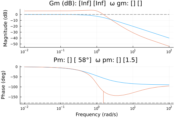
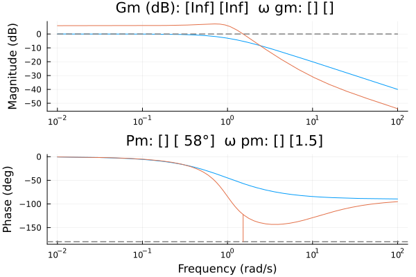
The "Nyquist freq." marker was drawn at 0.5 in both Bode plots on this page,
but the bodeplot x-axis is rad/s, so for Ts = 1 the Nyquist frequency is
pi/Ts ~ 3.14 rad/s. 0.5 is the Nyquist frequency expressed in Hz, off by a
factor 2*pi. Elsewhere on the same page the text already states "Nyquist
frequency is pi rad/s", so the page was internally inconsistent. Both markers
now use pi/Ts.

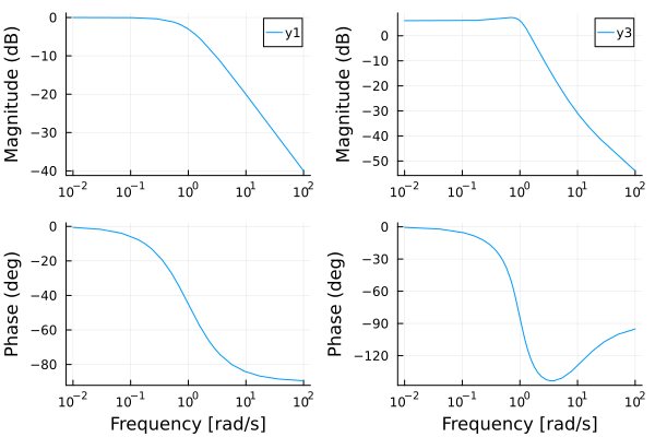
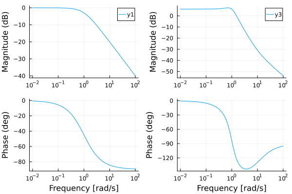
The first plot also only extended to omega = 1 rad/s, i.e. 0.32x the actual
Nyquist frequency. Over that range P(s)Z(s) and Pd(z) agree to within 0.4%,
which is invisible on a log-magnitude Bode plot, and the page concluded from
this that the two "match exactly". They do not. ZoH sampling folds the
response at all frequencies omega + k*omega_s down onto omega, so the exact
relation is the aliasing sum

    Pd(exp(i*omega*Ts)) = sum_k Z(i(omega + k*omega_s)) P(i(omega + k*omega_s))

of which P(s)Z(s) is only the k = 0 term. For the example on this page the
k = 0 truncation is within 1% up to 0.39x the Nyquist frequency, is off by
10% at omega = 2, and by 269% at 0.95x Nyquist. The frequency axis now runs
up to the Nyquist frequency so the divergence is visible, and the text states
the aliasing sum and points to d2c_exact for accurate work near Nyquist.

The same overstatement applied to the continuous-sinusoid time-domain
comparison further down (the amplitudes differ by ~1% at the input frequency
used there), so that claim is softened too.

The corresponding claim about d2c_exact is correct and is left unchanged --
it matches the discrete frequency response to ~1e-14 over the whole axis,
including above Nyquist, since it is an algebraic substitution.

Co-Authored-By: Claude Opus 5 (1M context) <noreply@anthropic.com>
Claude-Session: https://claude.ai/code/session_01VaQczXaXuF3KW5Lu9yMMD8

|
This is an automated message.
|

baggepinnen
marked this pull request as ready for review
July 31, 2026 10:12
This file contains hidden or bidirectional Unicode text that may be interpreted or compiled differently than what appears below. To review, open the file in an editor that reveals hidden Unicode characters.
Learn more about bidirectional Unicode characters
Sign up for free
to join this conversation on GitHub.
Already have an account?
Sign in to comment
2 participants


Add this suggestion to a batch that can be applied as a single commit.This suggestion is invalid because no changes were made to the code.Suggestions cannot be applied while the pull request is closed.Suggestions cannot be applied while viewing a subset of changes.Only one suggestion per line can be applied in a batch.Add this suggestion to a batch that can be applied as a single commit.Applying suggestions on deleted lines is not supported.You must change the existing code in this line in order to create a valid suggestion.Outdated suggestions cannot be applied.This suggestion has been applied or marked resolved.Suggestions cannot be applied from pending reviews.Suggestions cannot be applied on multi-line comments.Suggestions cannot be applied while the pull request is queued to merge.Suggestion cannot be applied right now. Please check back later.
Draft. Three related fixes to
docs/src/examples/zoh.md.1. The Nyquist frequency marker was off by a factor of 2π
Both Bode plots on the page draw the marker with
vline!([0.5 0.5], lab="Nyquist freq."). Thebodeplotx-axis is rad/s (hz=falseby default), so withTs = 1the Nyquist frequency isπ/Ts ≈ 3.14rad/s.0.5is that frequency in Hz.The page was already internally inconsistent about this — further down it says "(Nyquist frequency is π rad/s)", and
_default_freq_vectorinlib/ControlSystemsBase/src/freqresp.jluseslog10(π/sys.Ts)with the comment "Draw up to Nyquist frequency for discrete systems".Both markers now use
π/Ts.2.
P(s)Z(s)does not matchP_d(z)exactlyThe first plot only extended to
ω = 1rad/s — 0.32× the actual Nyquist frequency. Over that range the two agree to 0.4%, invisible on a log-magnitude plot, and the text concluded they "match exactly".They don't. ZoH sampling folds the response at every
ω + kω_sdown ontoω, so the exact relation is the aliasing sumand
P(s)Z(s)is only thek = 0term. Verified againstc2dto ~1e-14 relative error. For this page'sP = tf(0.1,[1,0.1,0.1]),Ts = 1, thek = 0truncation error is:P·ZThe frequency axis now runs up to the Nyquist frequency, which makes the divergence plainly visible, and the text states the aliasing sum and points to
d2c_exactfor work near Nyquist.Both plots become considerably more informative as a side effect — in the Discrete to continuous plot the marker now lands exactly on the fold, with the aliased image above it, which is what that section's prose is actually describing.
3. Same overstatement in the time domain
The continuous-sinusoid comparison said the output of
Pz"matches that ofPdexactly". At the input frequency used there the steady-state amplitudes differ by about 1% — the same aliasing contribution. Softened, and phrased without a hard-coded number so it does not go stale if the input frequency is changed.Left alone
The
d2c_exactclaim in the same file is correct and unchanged: it reproduces the discrete frequency response to ~1e-14 across the whole axis including above Nyquist, since it is an algebraicz^{-1} = e^{-sTs}substitution.Verification
Both edited
@exampleblocks were executed in a real session withControlSystems+Plotsand render as expected; the aliasing sum, the truncation errors, and thed2c_exactexactness were each checked numerically. I did not run a fulldocs/make.jlbuild (that environment needs Ipopt/GCMAES/etc.), but the only new Documenter construct is a same-page section@ref, a pattern already used elsewhere in these docs, andmakedocshere setswarnonly = [:missing_docs, :cross_references].🤖 Generated with Claude Code
https://claude.ai/code/session_01VaQczXaXuF3KW5Lu9yMMD8